Lake Urmia was the second largest permanent hyper-saline lake in the World and the biggest in Middle East. The alerting situation of the lake pushed the authority such that the United Nations declared it as the wetland of international importance and World’s biosphere reserve. In late 1990’s water level in the lake started to decline with a sharp trend such that a wasteland of salty desert was conceptualized for the lake’s future. Many researchers around the world tried to model, suggest or decode the fact behind the lake’s atrophy mostly accused by miss-management, dam construction, development of agricultural zones, climate change etc. as the main reason for the lake atrophy.
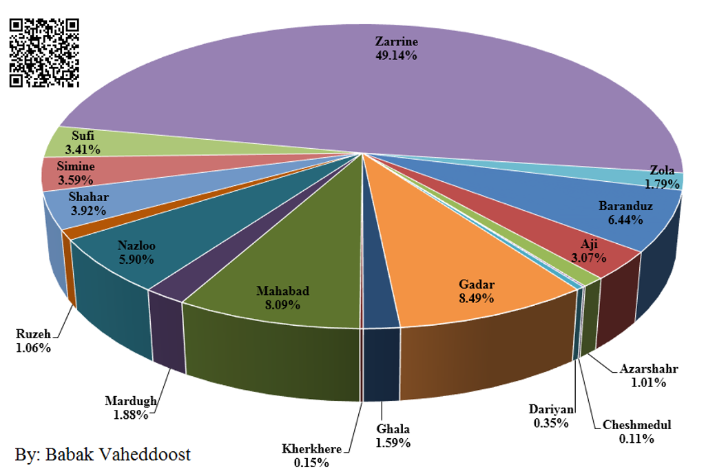
In this study, a lake water budget approach using hydro-meteorological variables; precipitation, evaporation, runoff and groundwater, was considered. For this aim, data from meteorological stations, stream-flow gauging stations and groundwater wells were gathered. Data were analyzed and a data inventory was obtained. The data inventory consists of 253 meteorological stations, 156 stream-flow gauging stations, 593 groundwater wells and 1 lake water level station all scattered over the Lake Urmia basin. Precipitation and evaporation were taken from meteorological stations. In this study, 7 meteorological stations, 18 stream-flow gauging stations and 9 groundwater wells were considered together with the lake water level station. The selected stations and groundwater wells are close to the lake and scatter around it.
Data in the selected stations and groundwater wells were checked against any missing data periods. Most of the stations were found with missing data. Groundwater wells have particularly long period of time with no data. For getting a common period for the analysis, missing data were reconstructed by a frequency domain analysis using decomposition. With this method, each time series of each station and groundwater well were decomposed into its components; trend, cycle, seasonality and randomness. An additive decomposition method was chosen. Observed time series was divided into calibration and validation parts. The decomposition method was used to fit a model to the calibration time series and to validate it then on the validation time series. Once validated, the model was run to reconstruct the missing data. This procedure was applied on all time series of precipitation, evaporation, runoff and groundwater. The observed and reconstructed precipitation, evaporation, runoff and groundwater time series were used to calculate lake water level. The calculated lake water level was compared with the observed lake water level. They were found in a very good agreement. This has been considered as a further validation of the reconstructed missing data.
Observed and reconstructed hydro-meteorological data were used together to develop models for forecasting lake water level. In the model, lake water depth was considered instead of lake water level. For this aim, two methods were combined. First, lake water depth was regressed on independent variables; precipitation, evaporation, runoff and groundwater. The second step is the development of stochastic model for each variable. Auto-regressive integrated moving average (ARIMA) models were used. A number of models were tested and finally the best models were determined based on performance criteria for each variable. The number of parameters was kept at minimum for the sake of parsimony. As the final step in the modeling, not hydro-meteorological variables (precipitation, evaporation, runoff and groundwater) but their selected stochastic models were inserted into the regression model developed at the very beginning step. This is defined as regressive-stochastic depth model.
Alternatively, difference in the lake water levels of two subsequent months was taken into account instead of the lake water depth when the regression model is developed in the first step. Because lake water depth can mask change in the lake water level as they have different orders of magnitudes.
From this study it is seen that Lake Urmia is under a serious atrophy problem that should be studied in a long-term interdisciplinary approach. Lake Urmia has a considerably well documented data although record periods without data may become problematic. The frequency domain analysis can be a tool to satisfactorily reconstruct the missing data in the hydro-meteorological time series. Lake water level models can be developed based on either lake water depth or the difference in the lake water level between subsequent months. Due to the order of magnitude difference between the depth and the depth difference, it is clear that depth models can mask the effect of each input variable; precipitation, evaporation, runoff and groundwater, on the lake water level. Therefore, depth difference models should be preferred for the sake of understanding the physical process in the lake water level precisely. Regressive-stochastic models were found successful in calculating the lake water level. In the proposed regressive-stochastic models, only previously observed hydro-meteorological data are needed. This is a good opportunity for one to be able to estimate the next month lake water level. This will help us decision makers to act in advance.
As a future suggestion, the lake and its watershed should be investigated through an interdisciplinary approach. As the change is a continuous process it is suggested that any model proposed should be revised every several years and/or after any major change happens in the basin.